As a test case we consider the AAD calculation of the vega of a Bermudan Swaption (30Y in 40Y, with semi-annual exercise) under a LIBOR Market Model (40Y, semi-annual, 320 time-steps, 15000 paths). The model has 25600 independent instantaneous volatility parameters, resulting in 12640 effective vega sensitivities.

**Table 1:** Vega of a Bermudan Swaption in the LIBOR Market Model: Calculation times and memory usages for finite differences and backward algorithmic differentiation algorithms. LIBOR market model with 40 years of simulation, 15000 paths, 80 forward rates, 320 time discretization points (1.5 month simulation time step), resulting in 25600 theoretical model vegas.
algorithm	evaluation	derivative	memory usage
finite difference	2.0 s	25600 s (7 hours)	1.5 GB
efficient stochastic AAD	4.6 s	27 s	8.7 GB

Differentiation of the Exercise Boundary

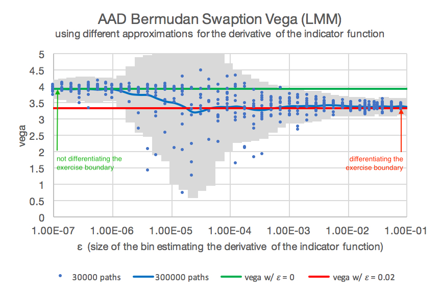BermudanSwaptionVega-AAD-with-DifferentBinSize

Figure 1: Vega of a Bermudan swaption using AAD for different values of $ \epsilon $ for the differentiation of the indicator function. The calculations were performed for 30000 paths with different bin sizes $ \epsilon $ (blue). We depict a mean (blue line) and standard deviation (grey). The green line marks the vega for $ \epsilon = 0 $ (ignoring the differentiation of the indicator function). The red line marks the vega for $ \epsilon = 0.2 $.

Differentiation of the expectation of Monte-Carlo samplings (simulations) involving indicator function appears in many financial products like barriers, digital options, Bermudan options and xVAs. The finite difference approximation of the differentiation results in unstable / noise values.

Although Bermudan options are (in an ideal situation) based on an optimal exercise, the differentiation of the indicator function is relevant, given that the estimation of the exercise boundary is not optimal.

We show that the AD applied to indicator functions in a Monte-Carlo valuation can be re-interpreted as a conditional expectation, which can be efficiently approximated: \[ \mathrm{E}\left( A \frac{\partial}{\partial X} \mathbb{1}(X > 0) \right) \ = \ \mathrm{E}\left( A \ \vert \ \{ X = 0 \} \right) \ \approx \ \mathrm{E}\left( A \frac{1}{2\delta} \mathbb{1}(|X| < \delta) \right) \text{.} \]

This allows for a local adaptive (per exercise boundary) choice of the approximation bin, e.g. using \[ 2 \delta \ = \ \epsilon \cdot \left( \mathrm{E}\left( X^{2} \right) \right)^{\frac{1}{2}} \]

To analyse the numerical stability, we depict the values of a parallel vega of the Bermudan swaption, where the conditional expectation is estimated by a least-square regression. In theory the differentiation of the conditional expectation could be ignored, since the Bermudan swaption valuation could assume optimal exercises (see Piterbarg 2004). However, the Monte-Carlo error and the regression error will result in a non-optimal exercise, which results in (slightly) a different vega. Assuming optimal exercise will result in wrong hedge ratios, since an exercise will be effectively sub-optimal due to the biased valuation of the future exercise dates. In addition, a comparison of the two different vegas (with and without ignoring differentiation of the indicator function) gives an indication of the quality of the conditional expectation estimator.

We may control the differentiation of the exercise boundary through the parameter $ \epsilon $ (where $ \epsilon=0 $ is interpreted as ignoring the differentiation of the indicator function). The parameter $ \epsilon $ thus enables us to investigate the optimality of each exercise boundary.

In Figure 1 we show the AAD vega for different values $ \epsilon $ for the size of the bin estimating the derivative of the indicator function. Since $ \epsilon $ determines the number of Monte-Carlo paths used for sampling the differentiation of the indicator functions, we see a larger Monte-Carlo error for very small epsilon. The value $ \epsilon=0 $ will switch off the differentiation of the indicator function and hence result in the AAD differentiation ignoring the differentiation of the indicator function. Small values of epsilon result in unstable vegas, since only few paths are used for the estimation. The value 0.2 can be interpreted statistically using 8% of the paths for the estimation of the derivative

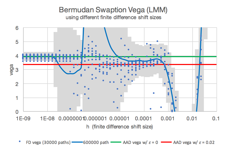Figure 2: Vega of a Bermudan swaption using finite differences (blue, different random number seeds and finite difference shifts). The red and green line mark the values obtained by AAD. The patterns visible for finite difference vegas are due to the same Monte-Carlo seed used for different shift sizes, generating a jump in vega once a Monte-Carlo path crosses the exercise boundary.

In Figure 2 we depict the classic, brute-force finite difference approximation of the vega for different shift sizes $ h $ and the stochastic AAD calculation of vega for $ \epsilon=0 $ (green) and $ \epsilon = 0.2 $ (red). We recover the effect that the finite difference approximation ignores the differentiation of the exercise boundary for very small shifts. This is due to the fact that under a small shift no path is crossing the exercise boundary. For larger shifts the finite difference approximation includes the differentiation of the exercise boundary, but results in a huge Monte-Carlo variance.

It is almost impossible to obtain a reliable estimate for the Bermudan swaption vega by finite differences, which includes the effect of a sub-optimal exercise by differentiation the indicator functions. AAD gives a reliable estimate (red). The finite difference sample points show some convergence to the correct solution for a narrow range of shifts sized $ h $ around 0.005.

Conclusion

Stochastic AAD enabled us to get a reliable estimate for the differentiation of the indicator function. For a Bermudan this is the differentiation of the exercise boundary, which matters if the estimator is non-optimal.

See https://ssrn.com/abstract=3000822 for details.

Delta of a Bermudan Digital Option

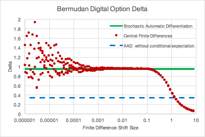Figure 3: Delta of a Bermudan digital option using different numerical methods:

Red: Central finite differences using different shift size (abscissa).
Green: Backward automatic differentiation applied to conditional expectation operator.
Blue: Backward automatic differentiation ignoring conditional expectation operator (will introduce a bias).

Remark: The calculations were repeated with 4 different Monte-Carlo random number seeds (hence there 4 red data series and 4 green data series (undistiguishable)).

As a test case we calculate the delta of a Bermudan digital option paying \[ \left\{ \begin{array}{ll} 1 & \text{ if } S(T_{i})-K_{i} > \tilde{U}(T_{i}) \text{ in $T_{i}$ and if no payout had been occurred before,} \\ 0 & \text{ otherwise, } \end{array} \right. \] where $ \tilde{U}(T) $ is the time $ T $ value of the future payoffs, for $ T_{1},\ldots,T_{n} $. Note that $ \tilde{U}(T_{n}) = 0 $, such that the last payment is a digital option.

This product is an ideal test-case: the valuation of $ \tilde{U}(T_{i}) $ is a conditional expectation. In addition, the conditional expectation only appears in the indicator function. The delta of a digital option payoff is only driven by the movement of the indicator function, since \[ \frac{\mathrm{d}}{\mathrm{d} S_{0}} \mathrm{E}( \mathbb{1}(f(S(T)) > 0) ) = \phi(f^{-1}(0)) \frac{\mathrm{d f(S)}}{\mathrm{d} S_{0}} \text{,} \] where $ \phi $ is the probability density of $ S $ and $ \mathbb{1}(\cdot) $ the indicator function. Hence, keeping the exercise boundary fixed, would result in a delta of 0.

We calculate the delta of a Bermudan digital option under a Black-Scholes model ( $ S_{0} = 1.0 $, $ r = 0.05 $, $ \sigma = 0.30 $ ) using 1000000 Monte-Carlo paths. We consider an option with $ T_{1} = 1 $, $ T_{2} = 2 $, $ T_{3} = 3 $, $ T_{4} = 4 $, and $ K_{1} = 0.5 $, $ K_{2} = 0.6 $, $ K_{3} = 0.8 $, $ K_{4} = 1.0 $. The implementation of this test case is available in finmath-lib-automaticdifferentiation-extensions. The results are depicted in Figure 3.

The finite difference approximation is biased for large shifts size The blue dashed line depicts the value of the delta of the conditional expectation operator is ignored. This generates a bias du to the correlation of derivative and underlying.

Forward Sensitivities

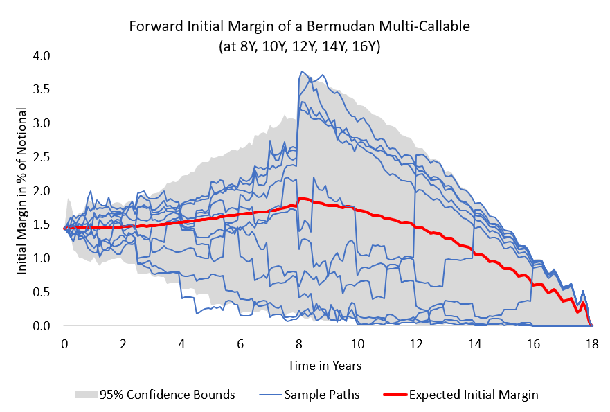Figure 4: Forward initial margin paths of a Bermudan callable swaption. For more results see https://ssrn.com/abstract=3095619 (results prepared by M. Viehmann)

Blue: Selected forward initial margin paths.
Red: Expected forward initial margin.
Grey: Standard deviation of the forward initial margin.

In https://ssrn.com/abstract=3018165 and https://ssrn.com/abstract=3095619 it is shown that we can derive all forward sensitivities in a single backward differentiation sweep (together with one conditional expectation estimation per time-step).

Forward sensitivities, sometimes called future sensitivities, are partial derivatives, at a future point in time. If $ V(t) $ denotes the time $ t $ value of a derivative product (or derivative portfolio) and $ X_{i}(t) $ ($ i=1,\ldots,r $) the time $ t $ values of the valuation model states (say, risk factors), then the forward sensitivities are \[ \frac{\partial V(t)}{\partial X_{i}(t)} \text{,} \quad i=1,\ldots,r \text{.} \]

Application: Hedge Simulation

A simple test for the accuracy of the forward simulation is a delta hedge: building up a portfolio consisting of $ \frac{\partial V(t, \omega)}{\partial S(t, \omega)} $ stocks (at every time step $ t $ and on every path $ \omega $ ) self-financing from a cash-account should result in replicating the final pay-off. Any mismatch in the sensitivities will result in replication error. This test can be performed without knowing an analytic benchmark for the forward sensitivities. We apply it to European and Bermudan options in https://ssrn.com/abstract=3095619.

Application: MVA from using ISDA-SIMM to construct the forward initial margin

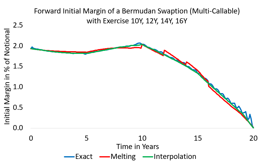Figure 5: Approximation methods for forward initial margins (here: expected forward initial margin) of a Bermudan callable swaption. For more results see https://ssrn.com/abstract=3095619 (results prepared by M. Viehmann)

Blue: Exact (AAD+ISDA SIMM based) forward initial margin.
Red: Melting ISDA SIMM sensitivities with selected reset dates.
Green: Interpolating sensitivities.

From the forward sensitivities we can construct an exact ISDA-SIMM forward initial margin and hence an exact ISDA-SIMM based MVA, see Figure 4. We use this as a benchmark to compare several method for fast(er) approximation of an forward sensitivity based MVA. See https://ssrn.com/abstract=3095619.

In this paper we consider several approximation methods for MVA from sensitivity based initial margin models (e.g. ISDA SIMM).

Computational Complexity

Automatic differentiation is not required to calculate forward sensitivities. However, backward mode differentiation has an advantage. Forward mode differentiation is only efficient if path-dependency is removed from the value process. Backward mode differentiation does not have this requirement.

With this in mind we have the following computational complexity:

Computational complexity assuming a Monte-Carlo simulation with $ n $-path, $ m $ time-steps and $ r $ risk factors, $ p $ basis functions for conditional expectations.
Computational complexity comparison
method	computational complexity
valuation
Monte-Carlo simulation	$ O(m \times n) $
all forward sensitivities
naive full re-simulation:	$ O(r \times m^2 \times n^2) $
forward mode differentiation:	$ O(r \times p^2 \times m \times n) $
backward mode differentiation:	$ O(1 \times p^2 \times m \times n) $

Note that $ n $ is very large (∼10000), $ m $ is large (∼100), $ r $ may be large (> 10) and $ p $ may be small.

See for details https://ssrn.com/abstract=3106068.

Stochastic Automatic Differentiation (Stochastic Algorithmic Differentiation)

Papers

Presentation Slides

Source Code